梯度下降：以二元线性回归为例

本文介绍用二元线性回归为引子，介绍三种梯度下降算法：批量梯度下降（batch gradient descent），随机梯度下降（stochastic gradient descent）和迷你批量梯度下降（mini batch gradient descent）

点击查看所需要的包

import numpy as np
from numpy.linalg import inv
import matplotlib
%matplotlib inline

import matplotlib.pyplot as plt
import matplotlib.patches as mpatches
from sklearn.linear_model import LinearRegression

正则方程组

线性回归预测模型的表示：
$$
\hat{y} = h_{\theta}(X) = X \cdot \theta
$$
通过最小化$\rm MSE$来训练模型：
$$
{\rm MSE}(X, h_{\theta}) = \frac{1}{m}\sum_{i=1}^{m} (\theta^T x^{(i)} - y^{(i)})^2
$$

使$\rm MSE$最小化的参数估计可用normal equation求出。

$$
\hat{\theta} = (X^T X)^{-1}X^T y
$$

使用normal equation的python范例

# ---- 用normal equation求模型参数 ----

# 生成测试用例
M = 100

x = 2 * np.random.rand(M, 1)              # 均匀分布
y = 4 + 3 * x + np.random.randn(M, 1)     # 正态分布

# 求模型参数
x_b = np.c_[np.ones((M, 1)), x]            # 补充上常数项bias
theta_hat = inv(x_b.T @ x_b) @ x_b.T @ y

theta_hat

array([[3.801864  ],
       [3.09766123]])

y_hat = x_b @ theta_hat

def example_plot(x, y, y_hat):
    fig1, ax = plt.subplots()
    ax.scatter(x, y, color='red', alpha=0.5)
    ax.plot(x, y_hat)
    plt.show()

example_plot(x, y, y_hat)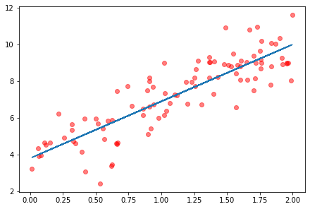

使用sklearn的例子：

lin_reg = LinearRegression()
lin_reg.fit(x, y)
lin_reg.intercept_, lin_reg.coef_

(array([3.801864]), array([[3.09766123]]))

三种梯度下降

梯度下降适合有大量feature或者过于大量instances的情况。

批量梯度下降

一次性计算cost function对所有参数的偏导数：

$$
\nabla_{\theta}{\rm MSE}(\theta) = \frac{2}{m}X^T(X\theta - y)
$$

偏导向量表示梯度下降的“方向”和“梯度”。从偏导向量可以得出下一步的参数向量：

$$
\theta^{\rm next} = \theta - \eta\nabla_{\theta}{\rm MSE}(\theta)
$$

其中$\eta$是learning rate学习速度。下面使用梯度下降拟合上面的数据。

首先，实现一个cost function，使用MSE作为cost function.

# implement cost function
def cost_mse(x, y, theta):
    m = len(y)
    h = x @ theta
    e = h - y
    mse = (1/m) * (e.T @ e)
    return mse

然后，通过梯度下降，传入一个theta，获得下一步的theta。

# batch update theta
def gradient_update(x, y, theta, eta):
    m = len(y)
    h = x @ theta
    new =  theta - (eta/m)*(x.T @ (h - y))
    return new

实现批量梯度下降

# implement batch_gradient descent
def batch_descent(x, y, eta, n_iter, record_theta=False, theta_init=None):
    m, k = x.shape

    if not theta_init:
        theta = np.zeros((k, 1))
    else:
        theta = np.array(theta_init).reshape(k, 1)
        
    # ------------------------------------------------------main loop
    if record_theta==False:
        for iteration in range(n_iter):
            theta = gradient_update(x, y, theta, eta)
        return theta
    #-------------------------------------------------------end main loop
    
    else:
        cost_rec = np.zeros(n_iter + 1)
        theta_rec = np.zeros((n_iter + 1, k))
        # initial cost
        cost_rec[0] = cost_mse(x, y, theta)
        # initial theta
        theta_rec[0, :] = theta.flatten()
        for iteration in range(n_iter):
            theta = gradient_update(x, y, theta, eta)
            cost_rec[iteration + 1] = cost_mse(x, y, theta)
            theta_rec[iteration + 1, :] = theta.flatten()
        return theta_rec, cost_rec

可视化批量梯度下降:

点击查看可视化的实现

# build contour map
class GradientContour(object):
    
    def __init__(self, fig, theta0grid, theta1grid, contour_level=30):
        self.theta0 = np.linspace(*theta0grid)
        self.theta1 = np.linspace(*theta1grid)
        self.len0 = len(self.theta0)
        self.len1 = len(self.theta1)
        self.theta0, self.theta1 = np.meshgrid(self.theta0, self.theta1)
        self.cost_val = np.zeros((self.len0, self.len1))
        self.colored = None
        self.fig = fig
        self.anno_colors = []
        
    def map_cost_val(self, x, y, cost_func): 
        for i in range(0, self.len0):
            for j in range(0, self.len1):
                theta_val = np.array((self.theta0[i,j], self.theta1[i,j])).reshape(2,1)
                self.cost_val[i,j] = cost_func(x, y, theta_val)
    
    def draw_blank_canvas(self, ax, x, y, cost_func, contour_level=30):
        self.map_cost_val(x, y, cost_func)
        ax.contour(self.theta0, self.theta1, self.cost_val, levels=contour_level,
                   colors='black', linestyles='dashed', linewidths=1)
        self.colored = ax.contourf(self.theta0, self.theta1, self.cost_val, levels=contour_level)
    
    def draw_gradients(self, ax, thetas, colorstr):
        self.anno_colors.append(colorstr)
        
        for i in range(0, len(thetas)-2):
            xstart, ystart = thetas[i+1]
            xend, yend = thetas[i]
                
            ax.annotate('', xy=(xstart, ystart), xytext=(xend, yend),
                        arrowprops={'arrowstyle':'-', 'color':colorstr, 'lw':2},
                        va='center', ha='center',
                        label = '')
    
    def graph_info(self, ax, xlabel, ylabel, title, show_legend=True):
        ax.set_xlabel(xlabel)
        ax.set_ylabel(ylabel, rotation=1)
        ax.set_title(title)
        if show_legend:
            plt.colorbar(self.colored, shrink=0.8)
            
    def add_label(self, labels):
        patches = []
        for i in range(len(self.anno_colors)):
            patch = mpatches.Patch(color=self.anno_colors[i], label=labels[i])
            patches.append(patch)
        plt.legend(handles=patches)
    
    def show_plot(self):
        self.fig.show()

eta    = 0.1    # learning rate
n_iter = 500    # num of iterations
thetas, costs = batch_descent(x_b, y, eta, n_iter, record_theta=True)

fig, ax = plt.subplots()
testplot = GradientContour(fig, theta0grid = (-1, 6, 30), theta1grid = (-1, 6, 30))
testplot.draw_blank_canvas(ax, x_b, y, cost_mse)
testplot.draw_gradients(ax, thetas, colorstr='red')
testplot.graph_info(ax, r'$\theta_0$', r'$\theta_1$', 'Contour map of univariate gradient descend')
testplot.add_label(['batch'])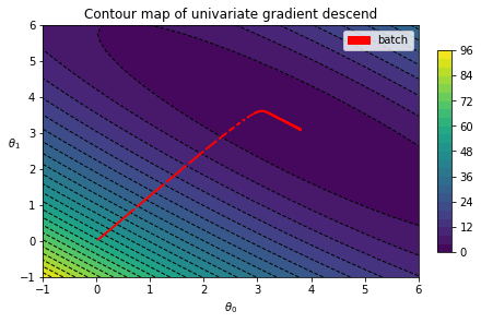

随机梯度下降

批量梯度下降遍历大小为m的数据集n_iters次，每次使用整个数据集更新theta。当样本较大时，这可能会导致训练速度过慢。随机梯度下降与之相反，每次只随机使用一条数据项更新theta。随机梯度下降遍历m大小的数据集n_epochs次，但往往可以以更小的n_epochs，更快的速度得到比较接近的结果。

由于随机只使用一条数据项更新theta，梯度下降的过程往往更为“到处游走”，可以想象某一步可能踏到很近最小值的点，但是下一步抽中了一个“离群点”，一步踏出最小值。一个解决方法是让learning rate随着迭代次数而逐步下降，越往后越难迈出大步。learning rate的变化方式被称为learning_schedule，下面是其中一个例子。

def learning_schedule(t, t0, t1):
    return t0 / (t + t1)

下面实现一个随机梯度下降函数。

def stochastic_descent(x, y, n_epochs, t0=5, t1=50, record_theta=False, theta_init=None):
    m, k = x.shape
    
    if not theta_init:
        theta = np.zeros((k, 1))
    else:
        theta = np.array(theta_init).reshape(k, 1)
    
    #---------------------------------------------main loop
    if record_theta == False:
        for epoch in range(n_epochs):
            for i in range(m):
                random_index = np.random.randint(m)
                xi = x[random_index : random_index+1]
                yi = y[random_index : random_index+1]
                eta = learning_schedule(epoch * m + i, t0, t1)
                theta = gradient_update(xi, yi, theta, eta)
        return theta
    #---------------------------------------------end loop
    
    else:
        cost_rec = np.zeros(n_epochs + 1)
        theta_rec = np.zeros((n_epochs + 1, k))
        # initial cost
        cost_rec[0] = cost_mse(x, y, theta)
        # initial theta
        theta_rec[0, :] = theta.flatten()
        for epoch in range(n_epochs):
            for i in range(m):
                random_index = np.random.randint(m)
                xi = x[random_index : random_index+1]
                yi = y[random_index : random_index+1]
                eta = learning_schedule(epoch * m + i, t0, t1)
                theta = gradient_update(xi, yi, theta, eta)
            cost_rec[epoch + 1] = cost_mse(x, y, theta)
            theta_rec[epoch + 1, :] = theta.flatten()
        return theta_rec, cost_rec

下面看梯度下降的路径。在这个例子里，最显著的特征是从初始值走的第一、二步走得非常大，直朝着最小值的方向。随后，再最小值附近，随机梯度下降不断地动荡。

n_epochs = 100
thetas, costs = stochastic_descent(x_b, y, n_epochs, record_theta=True, t0=10, t1=20)

fig, ax = plt.subplots()
testplot = GradientContour(fig, theta0grid = (-1, 6, 30), theta1grid = (-1, 6, 30))
testplot.draw_blank_canvas(ax, x_b, y, cost_mse)
testplot.draw_gradients(ax, thetas, colorstr='red')
testplot.graph_info(ax, r'$\theta_0$', r'$\theta_1$', 'Contour map of univariate gradient descend')
testplot.add_label(['stochastic'])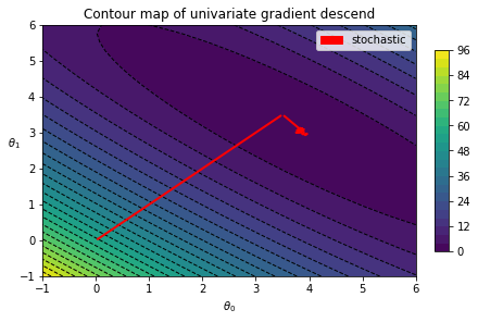

迷你批量梯度下降

迷你批量梯度下降是随机梯度下降（一次使用一条）和批量梯度下降（一次使用全部）的这种。

def mini_batch_descent(x, y, n_epochs, batch_size, t0=5, t1=50, record_theta=False, theta_init=None):
    m, k = x.shape
    
    if not theta_init:
        theta = np.zeros((k, 1))
    else:
        theta = np.array(theta_init).reshape(k, 1)

    x_y = np.concatenate((x, y), axis=1)
    #---------------------------------------------main loop
    if record_theta == False:
        for epoch in range(n_epochs):
            np.random.shuffle(x_y)
            x = x_y[:,:-1].reshape(m, k)
            y = x_y[:,-1].reshape(m, 1)
            for i in range(0, m, batch_size):
                xi = x[i : i+batch_size]
                yi = y[i : i+batch_size]
                eta = learning_schedule(epoch * m + i, t0, t1)
                theta = gradient_update(xi, yi, theta, eta)
        return theta
    #---------------------------------------------end loop
    
    else:
        cost_rec = np.zeros(n_epochs + 1)
        theta_rec = np.zeros((n_epochs + 1, k))
        # initial cost
        cost_rec[0] = cost_mse(x, y, theta)
        # initial theta
        theta_rec[0, :] = theta.flatten()
        for epoch in range(n_epochs):
            np.random.shuffle(x_y)
            x = x_y[:,:-1].reshape(m, k)
            y = x_y[:,-1].reshape(m, 1)
            for i in range(0, m, batch_size):
                xi = x[i : i+batch_size]
                yi = y[i : i+batch_size]
                eta = learning_schedule(epoch * m + i, t0, t1)
                theta = gradient_update(xi, yi, theta, eta)
            cost_rec[epoch + 1] = cost_mse(x, y, theta)
            theta_rec[epoch + 1, :] = theta.flatten()
        return theta_rec, cost_rec

从梯度下降的路线图可以看出，它没有随机梯度下降那么动荡，但收敛速度比批量梯度下降要快。

n_epochs = 100
batch_size = 4
thetas, costs = mini_batch_descent(x_b, y, n_epochs, batch_size, record_theta=True, t0=10, t1=20)

fig, ax = plt.subplots()
testplot = GradientContour(fig, theta0grid = (-1, 6, 30), theta1grid = (-1, 6, 30))
testplot.draw_blank_canvas(ax, x_b, y, cost_mse)
testplot.draw_gradients(ax, thetas, colorstr='red')
testplot.graph_info(ax, r'$\theta_0$', r'$\theta_1$', 'Contour map of univariate gradient descend')
testplot.add_label(['mini'])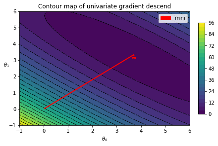

同时比较三种梯度下降方法。

batch_thetas, costs = batch_descent(x_b, y, eta=0.1, n_iter=500, record_theta=True)
stoch_thetas, costs = stochastic_descent(x_b, y, n_epochs=100, record_theta=True, t0=10, t1=20, theta_init=(2, 0))
mini_thetas, costs = mini_batch_descent(x_b, y, n_epochs=100, batch_size=4, record_theta=True, t0=10, t1=20, theta_init=(0,2))

fig, ax = plt.subplots(constrained_layout=False)
testplot = GradientContour(fig, theta0grid = (0, 5, 30), theta1grid = (0, 5, 30))
testplot.draw_blank_canvas(ax, x_b, y, cost_mse)
testplot.draw_gradients(ax, batch_thetas, colorstr='red')
testplot.draw_gradients(ax, stoch_thetas, colorstr='yellow')
testplot.draw_gradients(ax, mini_thetas, colorstr='white')
testplot.add_label(['batch','stoch','mini'])
testplot.graph_info(ax, r'$\theta_0$', r'$\theta_1$', 'Contour map of univariate gradient descend')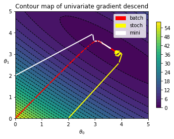

参考

• [1] Hnads-on Machine Learning with Scikit-Learn, Keras & TensorFlow, Aurelien Geron