sklearn机器学习：Classification

MNIST 数据库

导入MNIST数据库：

from sklearn.datasets import fetch_openml

mnist = fetch_openml("mnist_784", version=1)
mnist.keys()

dict_keys(['data', 'target', 'frame', 'categories', 'feature_names', 'target_names', 'DESCR', 'details', 'url'])

数据库关键字包括：

• DESCR： 描述数据库
• data: X数组，每行是一个instance，每列是一个feature
• target： y数组

x = mnist["data"].to_numpy()
y = mnist["target"].to_numpy()

print("x shape", x.shape)
print("y shape", y.shape)

x shape (70000, 784)
y shape (70000,)

一共有784个features，每个features表示一个像素点的灰度，每幅图像有$28\times28$个像素。

下面查看其中一个instance。

import matplotlib as mpl
import matplotlib.pyplot as plt

some_digit = x[0]
some_digit_image = some_digit.reshape(28, 28)

plt.imshow(some_digit_image, cmap="binary")
plt.axis("off")
plt.show()

y是以字符串形式储存的，所以要转换为整数类型。

import numpy as np

y = y.astype(np.int)

数据库已经预先“洗牌”并且划分好训练集（60,000）和测试集（10,000）:

x_train, x_test = x[:60000], x[60000:]
y_train, y_test = y[:60000], y[60000:]

训练一个binary classifier

以数字5为例，下面训练一个classifier，区分一个手写数字是5还是不是5。

创建一个关于数字是否是5的0/1向量：

y_train_5 = (y_train == 5)
y_test_5 = (y_test == 5)

使用SGD classifier训练模型:

from sklearn.linear_model import SGDClassifier

sgd_clf = SGDClassifier()        # random_state 相当于 seed
sgd_clf.fit(x_train, y_train_5)

SGDClassifier()

Try this classifier on some numbers.

sgd_clf.predict([some_digit])

array([ True])

Performance Measures

Measuring accuracy using cross-validation

from sklearn.model_selection import cross_val_score

cross_val_score(sgd_clf, x_train, y_train_5, cv=3, scoring="accuracy")

array([0.957  , 0.96095, 0.96665])

因为这个classifier只区分数字是不是5，而数据集中5只占10%，所以一个总是猜5以外的数字的分类器也能得到90%的准确率 – 和我们训练好的classifier没有表现出多大差距。

from sklearn.base import BaseEstimator

class Never5Classifier(BaseEstimator):
    '''
    这个分类器不会做任何拟合的努力
    这个分类器总是预测0
    '''
    def fit(self, x, y=None):
        pass
    def predict(self, x):
        return np.zeros((len(x), 1), dtype=bool)

下面来看看Never5Classifier的准确度：

never_5_clf = Never5Classifier()
cross_val_score(never_5_clf, x_train, y_train_5, cv=3, scoring="accuracy")

array([0.91125, 0.90855, 0.90915])

因此，准确度一般不是对classifier最好的分类标准。特别是对于一个skewed datasets（一些类别出现的频率远高于另一些频率时）。在此处。非5出现的频率远高于5的频率。

Confusion Matrix

from sklearn.model_selection import cross_val_predict

y_train_pred = cross_val_predict(sgd_clf, x_train, y_train_5, cv=3)

This returns the predictions made on each test fold. This means that you get a clean prediction for each instance in the training set. “Clean” means that the prediction is made by a model that never saw the data during training.

Now get the confusion matrix.

from sklearn.metrics import confusion_matrix

confusion_matrix(y_train_5, y_train_pred)

array([[53274,  1305],
       [ 1180,  4241]], dtype=int64)

Each row: an actual class.

Each col: a predicted class.

• 第一行第一列：属于非5，并预测非5的个数 (True Negative,TN)

• 第一行第二列，属于非5. 并预测为5的个数 (False Positive,FP)

• 第二行第一列，属于5. 并预测非5的个数 (False Negative,FN)

• 第二行第二列，属于5，并预测为5的个数 (True Positive,TP)

precision of the classifier: accuracy of the positive prediction:

$$
precision = \frac{TP}{TP+FP}
$$

recall, sensitivity or the true positive rate (TPR): ratio of positive instances that are correctly detected by the classifier:

$$
recall = \frac{TP}{TP+FN}
$$

from sklearn.metrics import precision_score, recall_score

precision = precision_score(y_train_5, y_train_pred)
recall = recall_score(y_train_5, y_train_pred)

print("Precision\t{:.4f}".format(precision))
print("Recall\t\t{:.4f}".format(recall))

Precision    0.7647
Recall        0.7823

$F_1$ score: harmonic mean of precision and recall classifier. The harmonic mean gives much more weight to low values. As a result, the classifier will only get a high $F_1$ score if both recall and precision are high.

$$
\begin{align}
F_1 = \frac{2}{\frac{1}{precision} + \frac{1}{recall}}
= 2 \times \frac{precision \times recall}{precision + recall}
= \frac{TP}{TP + \frac{FN + FP}{2}}
\end{align}
$$

from sklearn.metrics import f1_score

f1 = f1_score(y_train_5, y_train_pred)

print("F1\t{:.4f}".format(f1))

F1    0.7734

Precision/Recall Trade-off

Sometimes want high precision even if low recall:

儿童视频过滤器 – 提高阳性判定准确率，尽管意味着会有更多阳性实例被错过。

Sometimes want high recall even if low precision:

安保报警器 – 提高阳性实例被找到的概率，尽管这意味着阳性判断准确率会下降。

事实上， precision 和 recall 会存在一个权衡取舍的关系。在分类时，提高阳性门槛，会提高precision，但是降低recall，相反，降低阳性门槛会提高recall，但是可以提高阳性门槛。下面是人为为预测设定门槛的方法。

# access the decision score that the classifier uses to make decision
y_scores = sgd_clf.decision_function([some_digit])
y_scores

array([1039.78028102])

threshold = 0
y_some_digit_pred = (y_scores > threshold)
y_some_digit_pred

array([ True])

下面是选择threshold的方法。

首先，用cross_val_predict()函数获得所有训练集实例的预测值(clean)，但要求返回decision score而不是True/False的decision。

y_scores = cross_val_predict(sgd_clf, x_train, y_train_5, cv=3,
                             method="decision_function")

使用precision_recall_curve函数计算所有可能threshold的对应precision与recall。

from sklearn.metrics import precision_recall_curve

precisions, recalls, thresholds = precision_recall_curve(y_train_5, y_scores)

使用Matplotlib作图。

def plot_precision_recall_vs_threshold(precisions, recalls, thresholds):
    plt.plot(thresholds, precisions[:-1], "b--", label="Precision")
    plt.plot(thresholds, recalls[:-1], "g-", label="Recall")
    plt.legend()
    plt.xlabel("threshold")
    plt.ylim((0,1))
    plt.grid()

plot_precision_recall_vs_threshold(precisions, recalls, thresholds)
plt.show()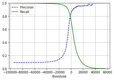

Precision在高threshold处呈现出一段bumpy的区间。这是因为，随着threshold的提高，能被认定阳性的案例减少，因而对于每一个错误都非常敏感。相反，在高threshold处，能被认定为阳性的案例已经很少了，再错漏一个不会有太大影响。

再分析在低threshold处，能被认定为阳性的案例很多，因此认错也多，再多认错一个敏感度不高，所以precision平滑；由于能被认定为阳性的案例很多，能找到的阳性基本都被找出来了，再少一个或者多一个，敏感度不大。

另一种方法：直接画出precision和recall的关系：

def plot_precision_vs_recall(precisions, recalls):
    plt.plot(recalls, precisions, "b-")
    plt.xlabel("Recall")
    plt.ylabel("Precision")
    plt.xlim((0,1))
    plt.ylim((0,1))
    plt.grid()
    
plot_precision_vs_recall(precisions, recalls)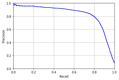

假如想要90% precision

threshold_90_precision = thresholds[np.argmax(precisions >= 0.90)]
threshold_90_precision

3056.0585000597052

y_train_pred_90 = (y_scores >= threshold_90_precision)

print("Precision\t{:.4f}".format(precision_score(y_train_5, y_train_pred_90)))
print("Recall\t\t{:.4f}".format(recall_score(y_train_5, y_train_pred_90)))

Precision    0.9000
Recall        0.5562

The ROC Curve

Receiver operating characteristics curve plots TPR against FPR.

TPR: True Positive Rate, or recall ratio – 在所有阳性案例中，识别出来阳性的比例。

$$
TPR = \frac{TP}{TP+FN}
$$

TNR: True Negative Rat, or specificity – 在所有阴性案例中，识别出来阴性的比例。

$$
TNR = \frac{TN}{TN+FP}
$$

FPR: False Positive Rate – 在所有阴性案例中，错误地识别出来阳性的比例（假阳性/所有阴性）

$$
FPR = 1-TNR
$$

所以ROC是sensitivity(recall) vs 1 - specificity – 真阳性/阳性 vs 假阳性/阴性

下面使用roc_curve()计算不同threshold下的TPR与FPR.

from sklearn.metrics import roc_curve

fpr, tpr, thresholds = roc_curve(y_train_5, y_scores) # y_scores: decision value

def plot_roc_curve(fpr, tpr, label=None):
    plt.plot(fpr, tpr, linewidth=2, label=label)
    plt.plot([0, 1], [0, 1], 'k--') # dashed diagonal
    plt.xlim((0,1))
    plt.ylim((0,1))
    plt.grid()
    plt.xlabel("False Positive Rate")
    plt.ylabel("True Positive Rate")

plot_roc_curve(fpr, tpr)
plt.show()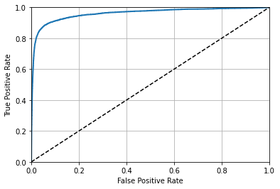

一个比较方法是比较AUC: area under the curve. 如果classifier是“完美的话”，FPR恒为0，TPR恒为1，AUC面积恒为1；如果classifier是随机的话，FPR = TPR，AUC面积接近0.5. 下面计算AUC。

from sklearn.metrics import roc_auc_score

print("AUC: {:.4f}".format(roc_auc_score(y_train_5, y_scores)))

AUC: 0.9604

如何选择Precision/recall (PR) curve或者AUC？

• PR:
  • positive class is rare
  • care more about the false positives than the false negatives
    （认定阳性时少出错）
• AUC:
  • positive class is not rare
  • care more about the false negatives than the false positives
    （尽量多地认出阳性）

Multi-class Classification

使用one-vs-one方法进行分类。

sgd_clf.fit(x_train, y_train) # 对所有类别进行分类
sgd_clf.predict([some_digit]) # 自动进行OvR的分类

array([5])

查看此实例对所有分类的decision value：

sgd_clf.decision_function([some_digit])

array([[-21024.40150978, -30404.40389192, -14057.76464372,
          1076.42126238, -24245.18237066,   3982.74400451,
        -21508.87615716, -14735.30165853,  -6727.9263852 ,
         -7748.15499922]])

交叉检验这个classifier的accuracy：分类正确的比例。

cross_val_score(sgd_clf, x_train, y_train, cv=3, scoring="accuracy")

array([0.88775, 0.87555, 0.8795 ])

Scaling the inputs 可以提高accuracy.

from sklearn.preprocessing import StandardScaler

scaler = StandardScaler()
x_train_scaled = scaler.fit_transform(x_train.astype(np.float64))
# cross_val_score(sgd_clf, x_train_scaled, y_train, cv=3, scoring="accuracy")

Error Analysis

假定已经获得一个最好的模型，现在想要提高这个模型。一个方法是分析它所犯的错误。

首先看它的confusion matrix。

y_train_pred = cross_val_predict(sgd_clf, x_train, y_train, cv=2)

conf_mx = confusion_matrix(y_train, y_train_pred)
conf_mx

array([[5637,    1,   32,   39,   11,   40,   37,    3,  104,   19],
       [   2, 6529,   25,   23,    7,   58,    5,   14,   69,   10],
       [  50,   92, 4909,  281,   51,   68,  106,   98,  277,   26],
       [  21,   38,  126, 5347,    5,  227,   11,   88,  193,   75],
       [  28,   32,   38,   30, 4757,   49,   84,   83,  179,  562],
       [  56,   23,   30,  327,   44, 4492,   82,   30,  261,   76],
       [  46,   27,   56,   60,   48,  234, 5311,    2,  126,    8],
       [  30,   32,   51,   54,   48,   38,    9, 5572,  108,  323],
       [  34,  160,   52,  241,   21,  415,   40,   40, 4727,  121],
       [  27,   20,   24,  100,  118,  124,    3,  220,  247, 5066]],
      dtype=int64)

利用灰度图可视化confusion matrix.

plt.matshow(conf_mx, cmap=plt.cm.gray)
plt.show()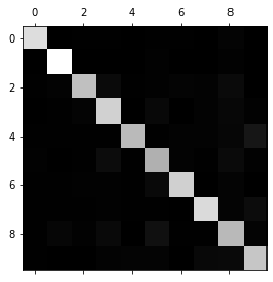

confusion matrix的每个元素都是instance的数量。现在把它标准化为比例。比如第二行第三列为把数字1（行）识别为数字2（列）的比例。

row_sums = conf_mx.sum(axis=1, keepdims=True)
norm_conf_mx = conf_mx / row_sums

把对角线元素都变为0，从而突出预测错误的情况。

np.fill_diagonal(norm_conf_mx, 0)
plt.matshow(norm_conf_mx, cmap=plt.cm.gray)
plt.show()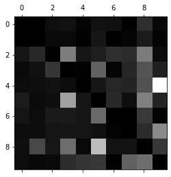

从图中可以看出，9经常被错误地认为是4，而4则往往能正确被识别出来。一个解决方法是针对性地收集更多“像4的9”，从而更好地训练模型分辨9和4。另外还有其他一些方法。

Multilabel Classification

指一个实例能分多个类的情况。

举例：创建一个classifier，给每个数据分配两个标签，第一个是大数与否（7， 8， 9属于大数），第二个是奇数与否。

from sklearn.neighbors import KNeighborsClassifier

y_train_large = (y_train >= 7)
y_train_odd = (y_train % 2 == 1)
y_multilabel = np.c_[y_train_large, y_train_odd]

knn_clf = KNeighborsClassifier()
knn_clf.fit(x_train, y_multilabel)

KNeighborsClassifier()

knn_clf.predict([some_digit])

array([[False,  True]])

y_train_knn_pred = cross_val_predict(knn_clf, x_train, y_multilabel, cv=3)

f1_score(y_multilabel, y_train_knn_pred, average="macro")

0.976410265560605

Multioutput Classification

输出多个标签（分类）；每个标签可以取多个值（而非只有0与1）。